Properties of graph components#
This section details the different attributes and properties which can be associated to nodes/neurons and connections in graphs and networks.
Content:
Components of a graph#
In the graph libraries used by NNGT, the main components of a graph are nodes (also called vertices in graph theory), which correspond to neurons in neural networks, and edges, which link nodes and correspond to synaptic connections between neurons in biology.
The library supposes for now that nodes/neurons and edges/synapses are always added and never removed. Because of this, we can attribute indices to the nodes and the edges which will be directly related to the order in which they have been created (the first node will have index 0, the second index 1, etc).
The source file for the examples given here can be found at doc/examples/attributes.py.
Node attributes#
If you are just working with basic graphs (for instance looking at the
influence of topology with purely excitatory networks), then your nodes do not
necessarily need to have attributes.
This is the same if you consider only the average effect of inhibitory neurons
by including inhibitory connections between the neurons but not a clear
distinction between populations of purely excitatory and purely inhibitory
neurons.
However, if you want to include additional information regarding the nodes, to
account for specific differences in their properties, then node attributes
are what you need. They are stored in node_attributes.
Furthermore, to model more realistic neuronal networks, you might also want to
define different groups and types of neurons, then connect them in specific
ways. This specific feature will be provides by NeuralGroup
objects.
Three types of node attributes#
In the library, there is a difference between:
standard attributes, which are stored in any type of
Graphand can be created, modified, and accessed via thenew_node_attribute(),set_node_attribute(), andget_node_attributes()functions.spatial properties (the positions of the neurons), which are stored in a specific
positionsnumpy.ndarrayand can be accessed using theget_positions()function,biological/group properties, which define assemblies of nodes sharing common properties, and are stored inside a
NeuralPopobject.
Standard attributes#
Standard attributes can be any given label that might vary among the nodes in the network and will be attached to each node.
Users can define any attribute, through the
new_node_attribute() function.
''' -------------- #
# Generate a graph #
# -------------- '''

num_nodes = 1000
avg_deg   = 25

graph = ng.erdos_renyi(nodes=num_nodes, avg_deg=avg_deg)


''' ----------------- #
# Add node attributes #
# ----------------- '''

# Let's make a network of animals where nodes represent either cats or dogs.
# (no discrimination against cats or dogs was intended, no animals were harmed
# while writing or running this code)
animals  = ["cat" for _ in range(600)]  # 600 cats
animals += ["dog" for _ in range(400)]  # and 400 dogs
np.random.shuffle(animals)              # which we assign randomly to the nodes

graph.new_node_attribute("animal", value_type="string", values=animals)
Attributes can have different types:
"double"for floating point numbers"int” for integers"string"for strings"object"for any other python object
Here we create a second node attribute of type "double":
# Nodes can have attributes of multiple types, let's add a size to our animals
catsizes = np.random.normal(50, 5, 600)   # cats around 50 cm
dogsizes = np.random.normal(80, 10, 400)  # dogs around 80 cm

# We first create the attribute without values (for "double", default to NaN)
graph.new_node_attribute("size", value_type="double")

# We now have to attributes: one containing strings, the other numbers (double)
print(graph.node_attributes)

# get the cats and set their sizes
cats = graph.get_nodes(attribute="animal", value="cat")
graph.set_node_attribute("size", values=catsizes, nodes=cats)

# We set 600 values so there are 400 NaNs left
assert np.sum(np.isnan(graph.get_node_attributes(name="size"))) == 400, \
    "There were not 400 NaNs as predicted."

# None of the NaN values belongs to a cat
assert not np.any(np.isnan(graph.get_node_attributes(cats, name="size"))), \
    "Got some cats with NaN size! :'("

# get the dogs and set their sizes
dogs = graph.get_nodes(attribute="animal", value="dog")
graph.set_node_attribute("size", values=dogsizes, nodes=dogs)
Biological/group properties#
Note
All biological/group properties are stored in a
NeuralPop object inside a Network
instance; this attribute can be accessed through
population.
NeuralPop objects can also be created from a
Graph or SpatialGraph but they will not be
stored inside the object.
The NeuralPop class allows you to define specific
groups of neurons (described by a NeuralGroup).
Once these populations are defined, you can constrain the connections between
those populations.
If the connectivity already exists, you can use the
GroupProperty class to create a population with
groups that respect specific constraints.
For more details on biological properties, see Groups, structures, and neuronal populations.
Edge attributes#
Like nodes, edges can also be attributed specific values to characterize them. However, where nodes are directly numbered and can be indexed and accessed easily, accessing edges is more complicated, especially since, usually, not all possible edges are present in a graph.
To easily access the desired edges, it is thus recommended to use the
get_edges() function.
Edge attributes can then be created and recovered using similar functions as
node attributes, namely new_edge_attribute(),
set_edge_attribute(), and
get_edge_attributes().
Weights and delays#
By default, graphs in NNGT are weighted: each edge is associated a “weight”
value (this behavior can be changed by setting weighted=False upon
creation).
Similarly, Network objects always have a “delay” associated to
their connections.
Both attributes can either be set upon graph creation, through the weights
and delays keyword arguments, or any any time using
set_weights() and set_delays().
Note
When working with NEST and using excitatory and inhibitory neurons via groups (see Groups, structures, and neuronal populations), the weight of all connections (including inhibitory connections) should be positive: the excitatory or inhibitory type of the synapses will be set automatically when the NEST network is created based on the type of the source neuron.
In general, it is also not a good idea to use negative weights directly
since standard graph analysis methods cannot handle them.
If you are not working with biologically realistic neurons and want to
set some inhibitory connections that do not depend on a “neuronal type”,
use the set_types() method.
Let us see how the get_edges() function can be used to
facilitate the creation of various weight patterns:
# Same as for node attributes, one can give attributes to the edges
# Let's give weights to the edges depending on how often the animals interact!
# cat's interact a lot among themselves, so we'll give them high weights
cat_edges = graph.get_edges(source_node=cats, target_node=cats)

# check that these are indeed only between cats
cat_set  = set(cats)
node_set = set(np.unique(cat_edges))

assert cat_set == node_set, "Damned, something wrong happened to the cats!"

# uniform distribution of weights between 30 and 50
graph.set_weights(elist=cat_edges, distribution="uniform",
                  parameters={"lower": 30, "upper": 50})

# dogs have less occasions to interact except some which spend a lot of time
# together, so we use a lognormal distribution
dog_edges = graph.get_edges(source_node=dogs, target_node=dogs)
graph.set_weights(elist=dog_edges, distribution="lognormal",
                  parameters={"position": 2.2, "scale": 0.5})

# Cats do not like dogs, so we set their weights to -5
# Dogs like chasing cats but do not like them much either so we let the default
# value of 1
cd_edges = graph.get_edges(source_node=cats, target_node=dogs)
graph.set_weights(elist=cd_edges, distribution="constant",
                  parameters={"value": -5})

# Let's check the distribution (you should clearly see 4 separate shapes)
if nngt.get_config("with_plot"):
    nngt.plot.edge_attributes_distribution(graph, "weight")
Note that here, the weights were generated randomly from specific distributions; for more details on the available distributions and their parameters, see Attributes and distributions.
Custom edge attributes#
Non-default edge attributes (besides “weights” or “delays”) can also be created through smilar functions as node attributes:
class Human:
    def __init__(self, name):
        self.name = name
    def __repr__(self):
        return "Human<{}>".format(self.name)

# let's create a class for humans and store it when two animals have interacted
# with the same human (the default will be an empty list if they did not)

# Alice interacted with all animals between 8 and 48
Alice   = Human("Alice")
animals = [i for i in range(8, 49)]
edges   = graph.get_edges(source_node=animals, target_node=animals)

graph.new_edge_attribute("common_interaction", value_type="object", val=[])
graph.set_edge_attribute("common_interaction", val=[Alice], edges=edges)

# Now suppose another human, Bob, interacted with all animals between 0 and 40
Bob     = Human("Bob")
animals = [i for i in range(0, 41)]
edges2  = graph.get_edges(source_node=animals, target_node=animals)

# to update the values, we need to get them to add Bob to the list
ci = graph.get_edge_attributes(name="common_interaction", edges=edges2)

for interactions in ci:
    interactions.append(Bob)

graph.set_edge_attribute("common_interaction", values=ci, edges=edges2)

# now some of the initial `edges` should have had their attributes updated
new_ci = graph.get_edge_attributes(name="common_interaction", edges=edges)
print(np.sum([0 if len(interaction) < 2 else 1 for interaction in new_ci]),
      "interactions have been updated among the", len(edges), "from Alice.")
Attributes and distributions#
Node and edge attributes can be generated based on the following distributions:
- uniform
a flat distribution with identical probability for all values,
parameters:
"lower"and"upper"values.
- delta
the Dirac delta “distribution”, where a single value can be drawn,
parameters:
"value".
- Gaussian
the normal distribution
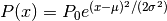
parameters:
"avg"( ) and
) and "std"( ).
).
- lognormal
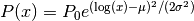
parameters:
"position"() and "scale"().
- linearly correlated
distribution name:
"lin_corr"a distribution which evolves linearly between two values depending on the value of a reference variable
parameters:
"correl_attribute"(the reference variable, usually another attribute),"lower"and"upper", the minimum and maximum values.
Example#
Generating a graph with delays that are linearly correlated to the distance between nodes.
dmin = 1.
dmax = 8.

d = {
    "distribution": "lin_corr", "correl_attribute": "distance",
    "lower": dmin, "upper": dmax
}

g = nngt.generation.distance_rule(200., nodes=100, avg_deg=10, delays=d)
Go to other tutorials: