Analysis module#
Tools to analyze neuronal networks, using either their topological properties, their activity, or more importantly, taking both into account. See also Consistent tools for graph analysis for more details on consistent analysis across graph libraries.
Content#
|
Adjacency matrix of the graph. |
|
Yields all shortest paths from source to target. |
|
Returns the assortativity of the graph. |
|
Returns the average shortest path length between sources and targets. |
|
Bayesian Blocks Implementation |
|
Returns the normalized betweenness centrality of the nodes and edges. |
|
Betweenness distribution of a graph. |
|
Binning function providing automatic binning using Bayesian blocks in addition to standard linear and logarithmic uniform bins. |
|
Returns the closeness centrality of some nodes. |
|
Returns the connected component to which each node belongs. |
|
Degree distribution of a graph. |
|
Returns the diameter of the graph. |
|
Return the B2 coefficient for the neurons. |
|
Return the average firing rate for the neurons. |
|
Return a 2D sparse matrix, where: |
|
Returns the global clustering coefficient. |
Returns the undirected global clustering coefficient. |
|
|
Compute the local closure for each node, as defined in [Yin2019] as the fraction of 2-walks that are closed. |
|
Local (weighted directed) clustering coefficient of the nodes, ignoring self-loops. |
Returns the undirected local clustering coefficient of some nodes. |
|
|
Return node attributes for a set of nodes. |
|
Returns the number of inhibitory connections. |
Calculate the edge reciprocity of the graph. |
|
|
Returns the length of the shortest paths between sources`and `targets. |
|
Returns a shortest path between source`and `target. |
|
Returns the small-world propensity of the graph as first defined in [Muldoon2016]. |
|
Spectral radius of the graph, defined as the eigenvalue of greatest module. |
|
Returns the subgraph centrality for each node in the graph. |
|
Computes the total firing rate of the network from the spike times. |
|
Same as |
|
Returns the number or the strength (also called intensity) of triangles for each node. |
|
Returns the number or the strength (also called intensity) of triplets for each node. |
Details#
- nngt.analysis.adjacency_matrix(graph, types=False, weights=False)[source]#
Adjacency matrix of the graph.
- Parameters:
graph (
Graphor subclass) – Network to analyze.types (bool, optional (default: False)) – Whether the excitatory/inhibitory type of the connnections should be considered (only if the weighing factor is the synaptic strength).
weights (bool or string, optional (default: False)) – Whether weights should be taken into account; if True, then connections are weighed by their synaptic strength, if False, then a binary matrix is returned, if weights is a string, then the ponderation is the correponding value of the edge attribute (e.g. “distance” will return an adjacency matrix where each connection is multiplied by its length).
- Returns:
a
csr_matrix.
References
[gt-adjacency][nx-adjacency]
- nngt.analysis.all_shortest_paths(g, source, target, directed=None, weights=None, combine_weights='mean')[source]#
Yields all shortest paths from source to target. The algorithms returns an empty generator if there is no path between the nodes.
- Parameters:
g (
Graph) – Graph to analyze.source (int) – Node from which the paths starts.
target (int, optional (default: all nodes)) – Node where the paths ends.
directed (bool, optional (default:
g.is_directed())) – Whether the edges should be considered as directed or not (automatically set to False if g is undirected).weights (str or array, optional (default: binary)) – Whether to use weighted edges to compute the distances. By default, all edges are considered to have distance 1.
combine_weights (str, optional (default: ‘mean’)) – How to combine the weights of reciprocal edges if the graph is directed but directed is set to False. It can be:
“sum”: the sum of the edge attribute values will be used for the new edge.
“mean”: the mean of the edge attribute values will be used for the new edge.
“min”: the minimum of the edge attribute values will be used for the new edge.
“max”: the maximum of the edge attribute values will be used for the new edge.
- Returns:
all_paths (generator) – Generator yielding paths as lists of ints.
References
- nngt.analysis.assortativity(g, degree, weights=None)[source]#
Returns the assortativity of the graph. This tells whether nodes are preferentially connected together depending on their degree.
- Parameters:
g (
Graph) – Graph to analyze.degree (str) – The type of degree that should be considered.
weights (bool or str, optional (default: binary edges)) – Whether edge weights should be considered; if
NoneorFalsethen use binary edges; ifTrue, uses the ‘weight’ edge attribute, otherwise uses any valid edge attribute required.
References
[nx-assortativity]networkx - algorithms.assortativity.degree_assortativity_coefficient
- nngt.analysis.average_path_length(g, sources=None, targets=None, directed=None, weights=None, combine_weights='mean', unconnected=False)[source]#
Returns the average shortest path length between sources and targets. The algorithms raises an error if all nodes are not connected unless unconnected is set to True.
The average path length is defined as
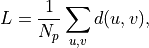
where
 is the number of paths between sources and targets,
and
is the number of paths between sources and targets,
and  is the shortest path distance from u to v.
If sources and targets are both None, then the total number of paths is
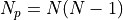 , with
  the number of nodes in the graph.
- Parameters:
g (
Graph) – Graph to analyze.sources (list of nodes, optional (default: all)) – Nodes from which the paths must be computed.
targets (list of nodes, optional (default: all)) – Nodes to which the paths must be computed.
directed (bool, optional (default:
g.is_directed())) – Whether the edges should be considered as directed or not (automatically set to False if g is undirected).weights (str or array, optional (default: binary)) – Whether to use weighted edges to compute the distances. By default, all edges are considered to have distance 1.
combine_weights (str, optional (default: ‘mean’)) – How to combine the weights of reciprocal edges if the graph is directed but directed is set to False. It can be:
“sum”: the sum of the edge attribute values will be used for the new edge.
“mean”: the mean of the edge attribute values will be used for the new edge.
“min”: the minimum of the edge attribute values will be used for the new edge.
“max”: the maximum of the edge attribute values will be used for the new edge.
unconnected (bool, optional (default: False)) – If set to true, ignores unconnected nodes and returns the average path length of the existing paths.
References
- nngt.analysis.bayesian_blocks(t, x=None, sigma=None, fitness='events', **kwargs)[source]#
Bayesian Blocks Implementation
This is a flexible implementation of the Bayesian Blocks algorithm described in Scargle 2012 [1]
Added in version 0.7.
- Parameters:
t (array_like) – data times (one dimensional, length N)
x (array_like (optional)) – data values
sigma (array_like or float (optional)) – data errors
fitness (str or object) – the fitness function to use. If a string, the following options are supported:
- ‘events’binned or unbinned event data
extra arguments are p0, which gives the false alarm probability to compute the prior, or gamma which gives the slope of the prior on the number of bins.
- ‘regular_events’non-overlapping events measured at multiples
of a fundamental tick rate, dt, which must be specified as an additional argument. The prior can be specified through gamma, which gives the slope of the prior on the number of bins.
- ‘measures’fitness for a measured sequence with Gaussian errors
The prior can be specified using gamma, which gives the slope of the prior on the number of bins. If gamma is not specified, then a simulation-derived prior will be used.
Alternatively, the fitness can be a user-specified object of type derived from the FitnessFunc class.
- Returns:
edges (ndarray) – array containing the (N+1) bin edges
Examples
Event data:
>>> t = np.random.normal(size=100)
>>> bins = bayesian_blocks(t, fitness='events', p0=0.01)
Event data with repeats:
>>> t = np.random.normal(size=100)
>>> t[80:] = t[:20]
>>> bins = bayesian_blocks(t, fitness='events', p0=0.01)
Regular event data:
>>> dt = 0.01
>>> t = dt * np.arange(1000)
>>> x = np.zeros(len(t))
>>> x[np.random.randint(0, len(t), len(t) / 10)] = 1
>>> bins = bayesian_blocks(t, fitness='regular_events', dt=dt, gamma=0.9)
Measured point data with errors:
>>> t = 100 * np.random.random(100)
>>> x = np.exp(-0.5 * (t - 50) ** 2)
>>> sigma = 0.1
>>> x_obs = np.random.normal(x, sigma)
>>> bins = bayesian_blocks(t, fitness='measures')
References
See also
astroML.plotting.hist()histogram plotting function which can make use of bayesian blocks.
- nngt.analysis.betweenness(g, btype='both', weights=None)[source]#
Returns the normalized betweenness centrality of the nodes and edges.
- Parameters:
g (
Graph) – Graph to analyze.btype (str, optional (default ‘both’)) – The centrality that should be returned (either ‘node’, ‘edge’, or ‘both’). By default, both betweenness centralities are computed.
weights (bool or str, optional (default: binary edges)) – Whether edge weights should be considered; if
NoneorFalsethen use binary edges; ifTrue, uses the ‘weight’ edge attribute, otherwise uses any valid edge attribute required.
- Returns:
nb (
numpy.ndarray) – The nodes’ betweenness if btype is ‘node’ or ‘both’eb (
numpy.ndarray) – The edges’ betweenness if btype is ‘edge’ or ‘both’
References
- nngt.analysis.betweenness_distrib(graph, weights=None, nodes=None, num_nbins='bayes', num_ebins='bayes', log=False)[source]#
Betweenness distribution of a graph.
- Parameters:
graph (
Graphor subclass) – the graph to analyze.weights (bool or str, optional (default: binary edges)) – Whether edge weights should be considered; if
NoneorFalsethen use binary edges; ifTrue, uses the ‘weight’ edge attribute, otherwise uses any valid edge attribute required.nodes (list or numpy.array of ints, optional (default: all nodes)) – Restrict the distribution to a set of nodes (only impacts the node attribute).
log (bool, optional (default: False)) – use log-spaced bins.
num_bins (int, list or str, optional (default: ‘bayes’)) – Any of the automatic methodes from
numpy.histogram(), or ‘bayes’ will provide automatic bin optimization. Otherwise, an int for the number of bins can be provided, or the direct bins list.
- Returns:
ncounts (
numpy.array) – number of nodes in each binnbetw (
numpy.array) – bins for node betweennessecounts (
numpy.array) – number of edges in each binebetw (
numpy.array) – bins for edge betweenness
- nngt.analysis.binning(x, bins='bayes', log=False)[source]#
Binning function providing automatic binning using Bayesian blocks in addition to standard linear and logarithmic uniform bins.
Added in version 0.7.
- Parameters:
x (array-like) – Array of data to be histogrammed
bins (int, list or ‘auto’, optional (default: ‘bayes’)) – If bins is ‘bayes’, in use bayesian blocks for dynamic bin widths; if it is an int, the interval will be separated into
log (bool, optional (default: False)) – Whether the bins should be evenly spaced on a logarithmic scale.
- nngt.analysis.closeness(g, weights=None, nodes=None, mode='out', harmonic=True, default=nan)[source]#
Returns the closeness centrality of some nodes.
Closeness centrality of a node u is defined, for the harmonic version, as the sum of the reciprocal of the shortest path distance
 from u to the N - 1 other nodes in the graph (if mode is “out”,
reciprocally
from u to the N - 1 other nodes in the graph (if mode is “out”,
reciprocally  , the distance to u from another node v,
if mode is “in”):
, the distance to u from another node v,
if mode is “in”):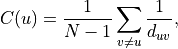
or, using the arithmetic definition, as the reciprocal of the average shortest path distance to/from u over to all other nodes:
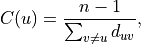
where d_{uv} is the shortest-path distance from u to v, and n is the number of nodes in the component.
By definition, the distance is infinite when nodes are not connected by a path in the harmonic case (such that
 ),
while the distance itself is taken as zero for unconnected nodes in the
first equation.
),
while the distance itself is taken as zero for unconnected nodes in the
first equation.- Parameters:
g (
Graph) – Graph to analyze.weights (bool or str, optional (default: binary edges)) – Whether edge weights should be considered; if
NoneorFalsethen use binary edges; ifTrue, uses the ‘weight’ edge attribute, otherwise uses any valid edge attribute required.nodes (list, optional (default: all nodes)) – The list of nodes for which the clutering will be returned
mode (str, optional (default: “out”)) – For directed graphs, whether the distances are computed from (“out”) or to (“in”) each of the nodes.
harmonic (bool, optional (default: True)) – Whether the arithmetic or the harmonic (recommended) version of the closeness should be used.
- Returns:
c (
numpy.ndarray) – The list of closeness centralities, on per node.
References
[nx-harmonic][nx-closeness]
- nngt.analysis.connected_components(g, ctype=None)[source]#
Returns the connected component to which each node belongs.
- Parameters:
g (
Graph) – Graph to analyze.ctype (str, optional (default ‘scc’)) – Type of component that will be searched: either strongly connected (‘scc’, by default) or weakly connected (‘wcc’).
- Returns:
cc, hist (
numpy.ndarray) – The component associated to each node (cc) and the number of nodes in each of the component (hist).
References
- nngt.analysis.degree_distrib(graph, deg_type='total', nodes=None, weights=None, log=False, num_bins='bayes')[source]#
Degree distribution of a graph.
- Parameters:
graph (
Graphor subclass) – the graph to analyze.deg_type (string, optional (default: “total”)) – type of degree to consider (“in”, “out”, or “total”).
nodes (list of ints, optional (default: None)) – Restrict the distribution to a set of nodes (default: all nodes).
weights (bool or str, optional (default: binary edges)) – Whether edge weights should be considered; if
NoneorFalsethen use binary edges; ifTrue, uses the ‘weight’ edge attribute, otherwise uses any valid edge attribute required.log (bool, optional (default: False)) – use log-spaced bins.
num_bins (int, list or str, optional (default: ‘bayes’)) – Any of the automatic methodes from
numpy.histogram(), or ‘bayes’ will provide automatic bin optimization. Otherwise, an int for the number of bins can be provided, or the direct bins list.
See also
- Returns:
counts (
numpy.array) – number of nodes in each bindeg (
numpy.array) – bins
- nngt.analysis.diameter(g, directed=None, weights=None, combine_weights='mean', is_connected=False)[source]#
Returns the diameter of the graph.
Changed in version 2.3: Added combine_weights argument.
Changed in version 2.0: Added directed and is_connected arguments.
It returns infinity if the graph is not connected (strongly connected for directed graphs) unless is_connected is True, in which case it returns the longest existing shortest distance.
- Parameters:
g (
Graph) – Graph to analyze.directed (bool, optional (default:
g.is_directed())) – Whether to compute the directed diameter if the graph is directed. If False, then the graph is treated as undirected. The option switches to False automatically if g is undirected.weights (bool or str, optional (default: binary edges)) – Whether edge weights should be considered; if
NoneorFalsethen use binary edges; ifTrue, uses the ‘weight’ edge attribute, otherwise uses any valid edge attribute required.combine_weights (str, optional (default: ‘mean’)) – How to combine the weights of reciprocal edges if the graph is directed but directed is set to False. It can be:
“sum”: the sum of the edge attribute values will be used for the new edge.
“mean”: the mean of the edge attribute values will be used for the new edge.
“min”: the minimum of the edge attribute values will be used for the new edge.
“max”: the maximum of the edge attribute values will be used for the new edge.
is_connected (bool, optional (default: False)) – If False, check whether the graph is connected or not and return infinite diameter if graph is unconnected. If True, the graph is assumed to be connected.
See also
References
[nx-diameter]
- nngt.analysis.get_b2(network=None, spike_detector=None, data=None, nodes=None)[source]#
Return the B2 coefficient for the neurons.
- Parameters:
network (
nngt.Network, optional (default: None)) – Network for which the activity was simulated.spike_detector (tuple of ints, optional (default: spike detectors)) – GID of the “spike_detector” objects recording the network activity.
data (array-like of shape (N, 2), optionale (default: None)) – Array containing the spikes data (first line must contain the NEST GID of the neuron that fired, second line must contain the associated spike time).
nodes (array-like, optional (default: all neurons)) – NNGT ids of the nodes for which the B2 should be computed.
- Returns:
b2 (array-like) – B2 coefficient for each neuron in nodes.
- nngt.analysis.get_firing_rate(network=None, spike_detector=None, data=None, nodes=None)[source]#
Return the average firing rate for the neurons.
- Parameters:
network (
nngt.Network, optional (default: None)) – Network for which the activity was simulated.spike_detector (tuple of ints, optional (default: spike detectors)) – GID of the “spike_detector” objects recording the network activity.
data (
numpy.arrayof shape (N, 2), optionale (default: None)) – Array containing the spikes data (first line must contain the NEST GID of the neuron that fired, second line must contain the associated spike time).nodes (array-like, optional (default: all nodes)) – NNGT ids of the nodes for which the B2 should be computed.
- Returns:
fr (array-like) – Firing rate for each neuron in nodes.
- nngt.analysis.get_spikes(recorder=None, spike_times=None, senders=None, astype='ssp')[source]#
Return a 2D sparse matrix, where:
each row i contains the spikes of neuron i (in NEST),
each column j contains the times of the jth spike for all neurons.
Changed in version 1.0: Neurons are now located in the row corresponding to their NEST GID.
- Parameters:
recorder (tuple, optional (default: None)) – Tuple of NEST gids, where the first one should point to the spike_detector which recorded the spikes.
spike_times (array-like, optional (default: None)) – If recorder is not provided, the spikes’ data can be passed directly through their spike_times and the associated senders.
senders (array-like, optional (default: None)) – senders[i] corresponds to the neuron which fired at spike_times[i].
astype (str, optional (default: “ssp”)) – Format of the returned data. Default is sparse lil_matrix (“ssp”) with one row per neuron, otherwise “np” returns a (T, 2) array, with T the number of spikes (the first row being the NEST gid, the second the spike time).
Example
>>> get_spikes()
>>> get_spikes(recorder)
>>> times = [1.5, 2.68, 125.6]
>>> neuron_ids = [12, 0, 65]
>>> get_spikes(spike_times=times, senders=neuron_ids)
Note
If no arguments are passed to the function, the first spike_recorder available in NEST will be used. Neuron positions correspond to their GIDs in NEST.
- Returns:
CSR matrix containing the spikes sorted by neuron GIDs (rows) and time
(columns).
- nngt.analysis.global_clustering(g, directed=True, weights=None, method='continuous', mode='total', combine_weights='mean')[source]#
Returns the global clustering coefficient.
This corresponds to the ratio of triangles to the number of triplets. For directed and weighted cases, see definitions of generalized triangles and triplets in the associated functions below.
- Parameters:
g (
Graph) – Graph to analyze.directed (bool, optional (default: True)) – Whether to compute the directed clustering if the graph is directed.
weights (bool or str, optional (default: binary edges)) – Whether edge weights should be considered; if
NoneorFalsethen use binary edges; ifTrue, uses the ‘weight’ edge attribute, otherwise uses any valid edge attribute required.method (str, optional (default: ‘continuous’)) – Method used to compute the weighted clustering, either ‘barrat’ [Barrat2004], ‘continuous’ [Fardet2021], ‘onnela’ [Onnela2005], or ‘zhang’ [Zhang2005].
mode (str, optional (default: “total”)) – Type of clustering to use for directed graphs, among “total”, “fan-in”, “fan-out”, “middleman”, and “cycle” [Fagiolo2007].
combine_weights (str, optional (default: ‘mean’)) – How to combine the weights of reciprocal edges if the graph is directed but directed is set to False. It can be:
“sum”: the sum of the edge attribute values will be used for the new edge.
“mean”: the mean of the edge attribute values will be used for the new edge.
“min”: the minimum of the edge attribute values will be used for the new edge.
“max”: the maximum of the edge attribute values will be used for the new edge.
Reference
———
.. [gt-global-clustering] :gtdoc:`clustering.global_clustering`
.. [ig-global-clustering] :igdoc:`transitivity_undirected`
.. [nx-global-clustering] :nxdoc:`algorithms.cluster.transitivity`
.. [Barrat2004] Barrat, Barthelemy, Pastor-Satorras, Vespignani. The – Architecture of Complex Weighted Networks. PNAS 2004, 101 (11). DOI: 10.1073/pnas.0400087101.
.. [Onnela2005] Onnela, Saramäki, Kertész, Kaski. Intensity and Coherence – of Motifs in Weighted Complex Networks. Phys. Rev. E 2005, 71 (6), 065103. DOI: 10.1103/physreve.71.065103, arxiv:cond-mat/0408629.
.. [Fagiolo2007] Fagiolo. Clustering in Complex Directed Networks. – Phys. Rev. E 2007, 76 (2), 026107. DOI: 10.1103/PhysRevE.76.026107, arXiv: physics/0612169.
.. [Zhang2005] Zhang, Horvath. A General Framework for Weighted Gene – Co-Expression Network Analysis. Statistical Applications in Genetics and Molecular Biology 2005, 4 (1). DOI: 10.2202/1544-6115.1128, PDF.
.. [Fardet2021] Fardet, Levina. Weighted directed clustering – interpretations and requirements for heterogeneous, inferred, and measured networks. 2021. arXiv: 2105.06318.
See also
- nngt.analysis.global_clustering_binary_undirected(g)[source]#
Returns the undirected global clustering coefficient.
This corresponds to the ratio of undirected triangles to the number of undirected triads.
- Parameters:
g (
Graph) – Graph to analyze.
References
[nx-global-clustering]
- nngt.analysis.local_closure(g, directed=True, weights=None, method=None, mode='cycle-out', combine_weights='mean')[source]#
Compute the local closure for each node, as defined in [Yin2019] as the fraction of 2-walks that are closed.
For undirected binary or weighted adjacency matrices
 , the normal (or Zhang-like) definition is given
by:
, the normal (or Zhang-like) definition is given
by: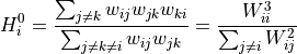
While a continuous version of the local closure is also proposed as:
![H_i = \frac{\sum_{j\neq k} \sqrt[3]{w_{ij} w_{jk} w_{ki}}^2}
{\sum_{j\neq k\neq i} \sqrt{w_{ij}w_{jk}}}
= \frac{\left( W^{\left[ \frac{2}{3} \right]} \right)_{ii}^3}
{\sum_{j \neq i} \left( W^{\left[ \frac{1}{2} \right]}
\right)^2_{ij}}](../_images/math/ce61fb6a10ab28c4c4643817103d858aab66aff5.png)
with
![W^{[\alpha]} = \{ w^\alpha_{ij} \}](../_images/math/c68763824a8a0af3bf2b09d0533649353af80ae0.png) .
.Directed versions of the local closure where defined as follow for a node
 connected to nodes
  and
and  :
:“cycle-out” is given by the pattern [(i, j), (j, k), (k, i)],
“cycle-in” is given by the pattern [(k, j), (j, i), (i, k)],
“fan-in” is given by the pattern [(k, j), (j, i), (k, i)],
“fan-out” is given by the pattern [(i, j), (j, k), (i, k)].
See [Fardet2021] for more details.
- Parameters:
g (
Graph) – Graph to analyze.directed (bool, optional (default: True)) – Whether to compute the directed clustering if the graph is directed.
weights (bool or str, optional (default: binary edges)) – Whether edge weights should be considered; if
NoneorFalsethen use binary edges; ifTrue, uses the ‘weight’ edge attribute, otherwise uses any valid edge attribute required.method (str, optional (default: ‘continuous’)) – Method used to compute the weighted clustering, either ‘normal’/’zhang’ or ‘continuous’.
mode (str, optional (default: “circle-out”)) – Type of clustering to use for directed graphs, among “circle-out”, “circle-in”, “fan-in”, or “fan-out”.
combine_weights (str, optional (default: ‘mean’)) – How to combine the weights of reciprocal edges if the graph is directed but directed is set to False. It can be:
“sum”: the sum of the edge attribute values will be used for the new edge.
“mean”: the mean of the edge attribute values will be used for the new edge.
“min”: the minimum of the edge attribute values will be used for the new edge.
“max”: the maximum of the edge attribute values will be used for the new edge.
References
[Yin2019] (1,2)Yin, Benson, and Leskovec. The Local Closure Coefficient: A New Perspective On Network Clustering. Proceedings of the Twelfth ACM International Conference on Web Search and Data Mining 2019, 303-311. DOI: 10.1145/3289600.3290991, PDF.
[Fardet2021]Fardet, Levina. Weighted directed clustering: interpretations and requirements for heterogeneous, inferred, and measured networks. 2021. arXiv: 2105.06318.
- nngt.analysis.local_clustering(g, nodes=None, directed=True, weights=None, method='continuous', mode='total', combine_weights='mean')[source]#
Local (weighted directed) clustering coefficient of the nodes, ignoring self-loops.
If no weights are requested and the graph is undirected, returns the undirected binary clustering.
For all weighted cases, the weights are assumed to be positive and they are normalized to dimensionless values between 0 and 1 through a division by the highest weight.
The default method for weighted networks is the continuous definition [Fardet2021] and is defined as:
![C_i = \frac{\sum_{jk} \sqrt[3]{w_{ij} w_{ik} w_{jk}}}
{\sum_{j\neq k} \sqrt{w_{ij} w_{ik}}}
= \frac{\left(W^{\left[\frac{2}{3}\right]}\right)^3_{ii}}
{\left(s^{\left[\frac{1}{2}\right]}_i\right)^2 - s_i}](../_images/math/65dc4269d66313fff39c57a052e948d6fd179462.png)
for undirected networks, with
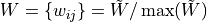 the normalized
weight matrix,
the normalized
weight matrix,  the normalized strength of node , and
![s^{[\frac{1}{2}]}_i = \sum_k \sqrt{w_{ik}}](../_images/math/b4993ffea0f6fc05f852fc3467f69c928253bb62.png) the strength associated
to the matrix
the strength associated
to the matrix ![W^{[\frac{1}{2}]} = \{\sqrt{w_{ij}}\}](../_images/math/81c8789346aca300ceb0c36499475cd6a2ea808d.png) .
.For directed networks, we used the total clustering defined in [Fagiolo2007] by default, hence the second equation becomes:
![C_i = \frac{\frac{1}{2}\left(W^{\left[\frac{2}{3}\right]}
+ W^{\left[\frac{2}{3}\right],T}\right)^3_{ii}}
{\left(s^{\left[\frac{1}{2}\right]}_i\right)^2
- 2s^{\leftrightarrow}_i - s_i}](../_images/math/22f259314b7c99d27f74cc02af706530290ac076.png)
with
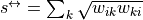 the
reciprocal strength (associated to reciprocal connections).
the
reciprocal strength (associated to reciprocal connections).For the other modes, see the generalized definitions in [Fagiolo2007].
Contrary to ‘barrat’ and ‘onnela’ [Saramaki2007], this method displays all following properties:
fully continuous (no jump in clustering when weights go to zero),
equivalent to binary clustering when all weights are 1,
equivalence between no-edge and zero-weight edge cases,
normalized (always between zero and 1).
Using either ‘continuous’ or ‘zhang’ is usually recommended for weighted graphs, see the discussion in [Fardet2021] for details.
- Parameters:
g (
Graphobject) – Graph to analyze.nodes (array-like container with node ids, optional (default = all nodes)) – Nodes for which the local clustering coefficient should be computed.
directed (bool, optional (default: True)) – Whether to compute the directed clustering if the graph is directed.
weights (bool or str, optional (default: binary edges)) – Whether edge weights should be considered; if
NoneorFalsethen use binary edges; ifTrue, uses the ‘weight’ edge attribute, otherwise uses any valid edge attribute required.method (str, optional (default: ‘continuous’)) – Method used to compute the weighted clustering, either ‘barrat’ [Barrat2004]/[Clemente2018], ‘continuous’ [Fardet2021], ‘onnela’ [Onnela2005]/[Fagiolo2007], or ‘zhang’ [Zhang2005].
mode (str, optional (default: “total”)) – Type of clustering to use for directed graphs, among “total”, “fan-in”, “fan-out”, “middleman”, and “cycle” [Fagiolo2007].
combine_weights (str, optional (default: ‘mean’)) – How to combine the weights of reciprocal edges if the graph is directed but directed is set to False. It can be:
“min”: the minimum of the edge attribute values will be used for the new edge.
“max”: the maximum of the edge attribute values will be used for the new edge.
“mean”: the mean of the edge attribute values will be used for the new edge.
“sum”: equivalent to mean due to weight normalization.
- Returns:
lc (
numpy.ndarray) – The list of clustering coefficients, on per node.
References
[Barrat2004]Barrat, Barthelemy, Pastor-Satorras, Vespignani. The Architecture of Complex Weighted Networks. PNAS 2004, 101 (11). DOI: 10.1073/pnas.0400087101.
[Clemente2018]Clemente, Grassi. Directed Clustering in Weighted Networks: A New Perspective. Chaos, Solitons & Fractals 2018, 107, 26–38. DOI: 10.1016/j.chaos.2017.12.007, arXiv: 1706.07322.
[Fagiolo2007]Fagiolo. Clustering in Complex Directed Networks. Phys. Rev. E 2007, 76, (2), 026107. DOI: 10.1103/PhysRevE.76.026107, arXiv: physics/0612169.
[Onnela2005]Onnela, Saramäki, Kertész, Kaski. Intensity and Coherence of Motifs in Weighted Complex Networks. Phys. Rev. E 2005, 71 (6), 065103. DOI: 10.1103/physreve.71.065103, arXiv: cond-mat/0408629.
[Saramaki2007]Saramäki, Kivelä, Onnela, Kaski, Kertész. Generalizations of the Clustering Coefficient to Weighted Complex Networks. Phys. Rev. E 2007, 75 (2), 027105. DOI: 10.1103/PhysRevE.75.027105, arXiv: cond-mat/0608670.
[Zhang2005]Zhang, Horvath. A General Framework for Weighted Gene Co-Expression Network Analysis. Statistical Applications in Genetics and Molecular Biology 2005, 4 (1). DOI: 10.2202/1544-6115.1128, PDF.
[Fardet2021]Fardet, Levina. Weighted directed clustering: interpretations and requirements for heterogeneous, inferred, and measured networks. 2021. arXiv: 2105.06318.
See also
undirected_binary_clustering(),global_clustering()
- nngt.analysis.local_clustering_binary_undirected(g, nodes=None)[source]#
Returns the undirected local clustering coefficient of some nodes.
If g is directed, then it is converted to a simple undirected graph (no parallel edges).
- Parameters:
g (
Graph) – Graph to analyze.nodes (list, optional (default: all nodes)) – The list of nodes for which the clustering will be returned
- Returns:
lc (
numpy.ndarray) – The list of clustering coefficients, on per node.
References
[nx-local-clustering]
- nngt.analysis.node_attributes(network, attributes, nodes=None, data=None)[source]#
Return node attributes for a set of nodes.
- Parameters:
network (
Graph) – The graph where the nodes belong.attributes (str or list) – Attributes which should be returned, among: * “betweenness” * “clustering” * “closeness” * “in-degree”, “out-degree”, “total-degree” * “subgraph_centrality”
nodes (list, optional (default: all nodes)) – Nodes for which the attributes should be returned.
data (
numpy.arrayof shape (N, 2), optional (default: None)) – Potential data on the spike events; if not None, it must contain the sender ids on the first column and the spike times on the second.
- Returns:
values (array-like or dict) – Returns the attributes, either as an array if only one attribute is required (attributes is a
str) or as adictof arrays.
- nngt.analysis.num_iedges(graph)[source]#
Returns the number of inhibitory connections.
For
Networkobjects, this corresponds to the number of edges stemming from inhibitory nodes (given bynngt.NeuralPop.inhibitory()). Otherwise, counts the edges where the type attribute is -1.
- nngt.analysis.reciprocity(g)[source]#
Calculate the edge reciprocity of the graph.
The reciprocity is defined as the number of edges that have a reciprocal edge (an edge between the same nodes but in the opposite direction) divided by the total number of edges. This is also the probability for any given edge, that its reciprocal edge exists. By definition, the reciprocity of undirected graphs is 1.
@todo: check whether we can get this for single nodes for all libraries.
- Parameters:
g (
Graph) – Graph to analyze.
References
[nx-reciprocity]
- nngt.analysis.shortest_distance(g, sources=None, targets=None, directed=None, weights=None, combine_weights='mean')[source]#
Returns the length of the shortest paths between sources`and `targets. The algorithms return infinity if there are no paths between nodes.
- Parameters:
g (
Graph) – Graph to analyze.sources (list of nodes, optional (default: all)) – Nodes from which the paths must be computed.
targets (list of nodes, optional (default: all)) – Nodes to which the paths must be computed.
directed (bool, optional (default:
g.is_directed())) – Whether the edges should be considered as directed or not (automatically set to False if g is undirected).weights (str or array, optional (default: binary)) – Whether to use weighted edges to compute the distances. By default, all edges are considered to have distance 1.
combine_weights (str, optional (default: ‘mean’)) – How to combine the weights of reciprocal edges if the graph is directed but directed is set to False. It can be:
“sum”: the sum of the edge attribute values will be used for the new edge.
“mean”: the mean of the edge attribute values will be used for the new edge.
“min”: the minimum of the edge attribute values will be used for the new edge.
“max”: the maximum of the edge attribute values will be used for the new edge.
- Returns:
distance (float, or 1d/2d numpy array of floats) – Distance (if single source and single target) or distance array. For multiple sources and targets, the shape of the matrix is (S, T), with S the number of sources and T the number of targets; for a single source or target, return a 1d-array of length T or S.
References
- nngt.analysis.shortest_path(g, source, target, directed=None, weights=None, combine_weights='mean')[source]#
Returns a shortest path between source`and `target. The algorithms returns an empty list if there is no path between the nodes.
- Parameters:
g (
Graph) – Graph to analyze.source (int) – Node from which the path starts.
target (int) – Node where the path ends.
directed (bool, optional (default:
g.is_directed())) – Whether the edges should be considered as directed or not (automatically set to False if g is undirected).weights (str or array, optional (default: binary)) – Whether to use weighted edges to compute the distances. By default, all edges are considered to have distance 1.
combine_weights (str, optional (default: ‘mean’)) – How to combine the weights of reciprocal edges if the graph is directed but directed is set to False. It can be:
“sum”: the sum of the edge attribute values will be used for the new edge.
“mean”: the mean of the edge attribute values will be used for the new edge.
“min”: the minimum of the edge attribute values will be used for the new edge.
“max”: the maximum of the edge attribute values will be used for the new edge.
- Returns:
path (list of ints) – Order of the nodes making up the path from source to target.
References
- nngt.analysis.small_world_propensity(g, directed=None, use_global_clustering=False, use_diameter=False, weights=None, combine_weights='mean', clustering='continuous', lattice=None, random=None, return_deviations=False)[source]#
Returns the small-world propensity of the graph as first defined in [Muldoon2016].
![\phi = 1 - \sqrt{\frac{\Pi_{[0, 1]}(\Delta_C^2) + \Pi_{[0, 1]}(\Delta_L^2)}{2}}](../_images/math/299cb35b8df9a39286a3209511c717fbf1dfeef4.png)
with
 the clustering deviation, i.e. the relative global or
average clustering of g compared to two reference graphs
the clustering deviation, i.e. the relative global or
average clustering of g compared to two reference graphs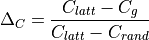
and
 the deviation of the average path length or diameter,
i.e. the relative average path length of g compared to that of the
reference graphs
the deviation of the average path length or diameter,
i.e. the relative average path length of g compared to that of the
reference graphs
In both cases, latt and rand refer to the equivalent lattice and Erdos-Renyi (ER) graphs obtained by rewiring g to obtain respectively the highest and lowest combination of clustering and average path length.
Both deviations are clipped to the [0, 1] range in case some graphs have a higher clustering than the lattice or a lower average path length than the ER graph.
- Parameters:
g (
Graphobject) – Graph to analyze.directed (bool, optional (default: True)) – Whether to compute the directed clustering if the graph is directed. If False, then the graph is treated as undirected. The option switches to False automatically if g is undirected.
use_global_clustering (bool, optional (default: True)) – If False, then the average local clustering is used instead of the global clustering.
use_diameter (bool, optional (default: False)) – Use the diameter instead of the average path length to have more global information. Ccan also be much faster in some cases, especially using graph-tool as the backend.
weights (bool or str, optional (default: binary edges)) – Whether edge weights should be considered; if
NoneorFalsethen use binary edges; ifTrue, uses the ‘weight’ edge attribute, otherwise uses any valid edge attribute required.combine_weights (str, optional (default: ‘mean’)) – How to combine the weights of reciprocal edges if the graph is directed but directed is set to False. It can be:
“sum”: the sum of the edge attribute values will be used for the new edge.
“mean”: the mean of the edge attribute values will be used for the new edge.
“min”: the minimum of the edge attribute values will be used for the new edge.
“max”: the maximum of the edge attribute values will be used for the new edge.
clustering (str, optional (default: ‘continuous’)) – Method used to compute the weighted clustering coefficients, either ‘barrat’ [Barrat2004], ‘continuous’ (recommended), or ‘onnela’ [Onnela2005].
lattice (
nngt.Graph, optional (default: generated from g)) – Lattice to use as reference (since its generation is deterministic, enables to avoid multiple generations when running the algorithm several times with the same graph)random (
nngt.Graph, optional (default: generated from g)) – Random graph to use as reference. Can be useful for reproducibility or for very sparse graphs where ER algorithm would statistically lead to a disconnected graph.return_deviations (bool, optional (default: False)) – If True, the deviations are also returned, in addition to the small-world propensity.
Note
If weights are provided, the distance calculation uses the inverse of the weights. This implementation differs slightly from the original implementation as it can also use the global instead of the average clustering coefficient, the diameter instead of the avreage path length, and it is generalized to directed networks.
References
[Muldoon2016] (1,2)Muldoon, Bridgeford, Bassett. Small-World Propensity and Weighted Brain Networks. Sci Rep 2016, 6 (1), 22057. DOI: 10.1038/srep22057, arXiv: 1505.02194.
[Barrat2004]Barrat, Barthelemy, Pastor-Satorras, Vespignani. The Architecture of Complex Weighted Networks. PNAS 2004, 101 (11). DOI: 10.1073/pnas.0400087101.
[Onnela2005]Onnela, Saramäki, Kertész, Kaski. Intensity and Coherence of Motifs in Weighted Complex Networks. Phys. Rev. E 2005, 71 (6), 065103. DOI: 10.1103/physreve.71.065103, arxiv:cond-mat/0408629.
- Returns:
phi (float in [0, 1]) – The small-world propensity.
delta_l (float) – The average path-length deviation (if return_deviations is True).
delta_c (float) – The clustering deviation (if return_deviations is True).
- nngt.analysis.spectral_radius(graph, typed=True, weights=True)[source]#
Spectral radius of the graph, defined as the eigenvalue of greatest module.
- Parameters:
graph (
Graphor subclass) – Network to analyze.typed (bool, optional (default: True)) – Whether the excitatory/inhibitory type of the connnections should be considered.
weights (bool, optional (default: True)) – Whether weights should be taken into account, defaults to the “weight” edge attribute if present.
- Returns:
the spectral radius as a float.
- nngt.analysis.subgraph_centrality(graph, weights=True, nodes=None, normalize='max_centrality')[source]#
Returns the subgraph centrality for each node in the graph.
Defined according to [Estrada2005] as:

where
 is the (potentially weighted and normalized) adjacency
matrix.
is the (potentially weighted and normalized) adjacency
matrix.- Parameters:
graph (
Graphor subclass) – Network to analyze.weights (bool or string, optional (default: True)) – Whether weights should be taken into account; if True, then connections are weighed by their synaptic strength, if False, then a binary matrix is returned, if weights is a string, then the ponderation is the correponding value of the edge attribute (e.g. “distance” will return an adjacency matrix where each connection is multiplied by its length).
nodes (array-like container with node ids, optional (default = all nodes)) – Nodes for which the subgraph centrality should be returned (all centralities are computed anyway in the algorithm).
normalize (str or False, optional (default: “max_centrality”)) – Whether the centrality should be normalized. Accepted normalizations are “max_eigenvalue” (the matrix is divided by its largest eigenvalue), “max_centrality” (the largest centrality is one), and
Falseto get the non-normalized centralities.
- Returns:
centralities (
numpy.ndarray) – The subgraph centrality of each node.
References
[Estrada2005]Ernesto Estrada and Juan A. Rodríguez-Velázquez, Subgraph centrality in complex networks, PHYSICAL REVIEW E 71, 056103 (2005), DOI: 10.1103/PhysRevE.71.056103, arXiv: cond-mat/0504730.
- nngt.analysis.total_firing_rate(network=None, spike_detector=None, nodes=None, data=None, kernel_center=0.0, kernel_std=30.0, resolution=None, cut_gaussian=5.0)[source]#
Computes the total firing rate of the network from the spike times. Firing rate is obtained as the convolution of the spikes with a Gaussian kernel characterized by a standard deviation and a temporal shift.
Added in version 0.7.
- Parameters:
network (
nngt.Network, optional (default: None)) – Network for which the activity was simulated.spike_detector (tuple of ints, optional (default: spike detectors)) – GID of the “spike_detector” objects recording the network activity.
data (
numpy.arrayof shape (N, 2), optionale (default: None)) – Array containing the spikes data (first line must contain the NEST GID of the neuron that fired, second line must contain the associated spike time).kernel_center (float, optional (default: 0.)) – Temporal shift of the Gaussian kernel, in ms.
kernel_std (float, optional (default: 30.)) – Characteristic width of the Gaussian kernel (standard deviation) in ms.
resolution (float or array, optional (default: 0.1*kernel_std)) – The resolution at which the firing rate values will be computed. Choosing a value smaller than kernel_std is strongly advised. If resolution is an array, it will be considered as the times were the firing rate should be computed.
cut_gaussian (float, optional (default: 5.)) – Range over which the Gaussian will be computed. By default, we consider the 5-sigma range. Decreasing this value will increase speed at the cost of lower fidelity; increasing it with increase the fidelity at the cost of speed.
- Returns:
fr (array-like) – The firing rate in Hz.
times (array-like) – The times associated to the firing rate values.
- nngt.analysis.transitivity(g, directed=True, weights=None)[source]#
Same as
global_clustering().
- nngt.analysis.triangle_count(g, nodes=None, directed=True, weights=None, method='normal', mode='total', combine_weights='mean')[source]#
Returns the number or the strength (also called intensity) of triangles for each node.
- Parameters:
g (
Graphobject) – Graph to analyze.nodes (array-like container with node ids, optional (default = all nodes)) – Nodes for which the local clustering coefficient should be computed.
directed (bool, optional (default: True)) – Whether to compute the directed clustering if the graph is directed.
weights (bool or str, optional (default: binary edges)) – Whether edge weights should be considered; if
NoneorFalsethen use binary edges; ifTrue, uses the ‘weight’ edge attribute, otherwise uses any valid edge attribute required.method (str, optional (default: ‘normal’)) – Method used to compute the weighted triangles, either ‘normal’, where the weights are directly used, or the definitions associated to the weighted clustering: ‘barrat’ [Barrat2004], ‘continuous’, ‘onnela’ [Onnela2005], or ‘zhang’ [Zhang2005].
mode (str, optional (default: “total”)) – Type of clustering to use for directed graphs, among “total”, “fan-in”, “fan-out”, “middleman”, and “cycle” [Fagiolo2007].
combine_weights (str, optional (default: ‘mean’)) – How to combine the weights of reciprocal edges if the graph is directed but directed is set to False. It can be:
“sum”: the sum of the edge attribute values will be used for the new edge.
“mean”: the mean of the edge attribute values will be used for the new edge.
“min”: the minimum of the edge attribute values will be used for the new edge.
“max”: the maximum of the edge attribute values will be used for the new edge.
- Returns:
tr (array) – Number or weight of triangles to which each node belongs.
References
[Barrat2004]Barrat, Barthelemy, Pastor-Satorras, Vespignani. The Architecture of Complex Weighted Networks. PNAS 2004, 101 (11). DOI: 10.1073/pnas.0400087101.
[Fagiolo2007]Fagiolo. Clustering in Complex Directed Networks. Phys. Rev. E 2007, 76, (2), 026107. DOI: 10.1103/PhysRevE.76.026107, arXiv: physics/0612169.
[Onnela2005]Onnela, Saramäki, Kertész, Kaski. Intensity and Coherence of Motifs in Weighted Complex Networks. Phys. Rev. E 2005, 71 (6), 065103. DOI: 10.1103/physreve.71.065103, arXiv: cond-mat/0408629.
[Zhang2005]Zhang, Horvath. A General Framework for Weighted Gene Co-Expression Network Analysis. Statistical Applications in Genetics and Molecular Biology 2005, 4 (1). DOI: 10.2202/1544-6115.1128, PDF.
- nngt.analysis.triplet_count(g, nodes=None, directed=True, weights=None, method='normal', mode='total', combine_weights='mean')[source]#
Returns the number or the strength (also called intensity) of triplets for each node.
For binary networks, the triplets of node
are defined as:
- Parameters:
g (
Graphobject) – Graph to analyze.nodes (array-like container with node ids, optional (default = all nodes)) – Nodes for which the local clustering coefficient should be computed.
directed (bool, optional (default: True)) – Whether to compute the directed clustering if the graph is directed.
weights (bool or str, optional (default: binary edges)) – Whether edge weights should be considered; if
NoneorFalsethen use binary edges; ifTrue, uses the ‘weight’ edge attribute, otherwise uses any valid edge attribute required.method (str, optional (default: ‘continuous’)) – Method used to compute the weighted triplets, either ‘normal’, where the edge weights are directly used, or the definitions used for weighted clustering coefficients, ‘barrat’ [Barrat2004], ‘continuous’, ‘onnela’ [Onnela2005], or ‘zhang’ [Zhang2005].
mode (str, optional (default: “total”)) – Type of clustering to use for directed graphs, among “total”, “fan-in”, “fan-out”, “middleman”, and “cycle” [Fagiolo2007].
combine_weights (str, optional (default: ‘mean’)) – How to combine the weights of reciprocal edges if the graph is directed but directed is set to False. It can be:
“sum”: the sum of the edge attribute values will be used for the new edge.
“mean”: the mean of the edge attribute values will be used for the new edge.
“min”: the minimum of the edge attribute values will be used for the new edge.
“max”: the maximum of the edge attribute values will be used for the new edge.
- Returns:
tr (array) – Number or weight of triplets to which each node belongs.
References
[Barrat2004]Barrat, Barthelemy, Pastor-Satorras, Vespignani. The Architecture of Complex Weighted Networks. PNAS 2004, 101 (11). DOI: 10.1073/pnas.0400087101.
[Fagiolo2007]Fagiolo. Clustering in Complex Directed Networks. Phys. Rev. E 2007, 76, (2), 026107. DOI: 10.1103/PhysRevE.76.026107, arXiv: physics/0612169.
[Zhang2005]Zhang, Horvath. A General Framework for Weighted Gene Co-Expression Network Analysis. Statistical Applications in Genetics and Molecular Biology 2005, 4 (1). DOI: 10.2202/1544-6115.1128, PDF.